
Some Notes for Smoke and PYRO
Learning PYRO in Houdini is not an easy task. Unlike the SOP, it is established based on the real physic model. For a better understanding of how PYRO works, We have to know what is behind the scene.
Basics
The field in Smoke / Pyro solver
In fluid dynamics, there are two basic types of interpretation to describe how fluids move: Euler & lagrangian. Generally, the Lagrangian perspective is focusing on the object itself, and the Euler perspective is focusing on the "field." Due to the different aspects, those two methods are also called particle-based / grid-based methods.
Lagrangian v.s. Euler
Let take a look at the difference between the two methods. For example, suppose we have smoke moving in the air:
The Lagrangian perspective thinks the whole air as a static "container." The moving smoke is consists of tons of particles(like point cloud). They are moving independently, but affect adjacent particles at the same time. We store some information on per-particle (such as velocity, temperature, color) to control how the smoke moves. Analysis information that applied to those particles is sample since we only need to focus on tracking the particles individually from beginning to end. However, in fluid dynamics, calculate all the interactional data is impossible due to the insane amount of particles, especially when we try to keep the mass conservation in the movement.
Instead of taking all particles into account, the Euler perspective chooses to use the "field" to describe how smoke moves, that is, dividing the specified domain into the amount of 3d cells, which is called voxels. Each voxel store the data we need to describe the current status of the smoke. If we want to describe the whole movement, we have to update the data in each voxel every step(yep, it is the step we saw in Houdini). The updating process is called advection. It is much easier to provide mass conservation under Euler's viewpoint because we are no longer need to calculate the interaction forces between the units; The calculation has been reduced to the voxel level. That is, for every voxel, we have mass conservation if the amount of gas entering and exiting in the voxel were equal.
The Drawback of Euler's Method
The drawbacks of Euler representation are we lose data all the time during the simulation; that is a significant compromise when we use Euler's perspective to interpret the fluid movement.
Through the Helmholtz decomposition, any vector field can be sperate into two parts:
- Incompressible vector field, also known as the divergence-free vector filed.
- Conservative vector field, which is also known as the curl-free vector field.
In Euler's method, the Conservative vector field has been ignored, and it is the reason cause the simulation to lose data. For example, suppose we advect density by velocity. If the density exists between two voxels, to get the advection result, we need to perform some interpolation on both density field and velocity field. Thus, any details that exist between the two voxels have been blended.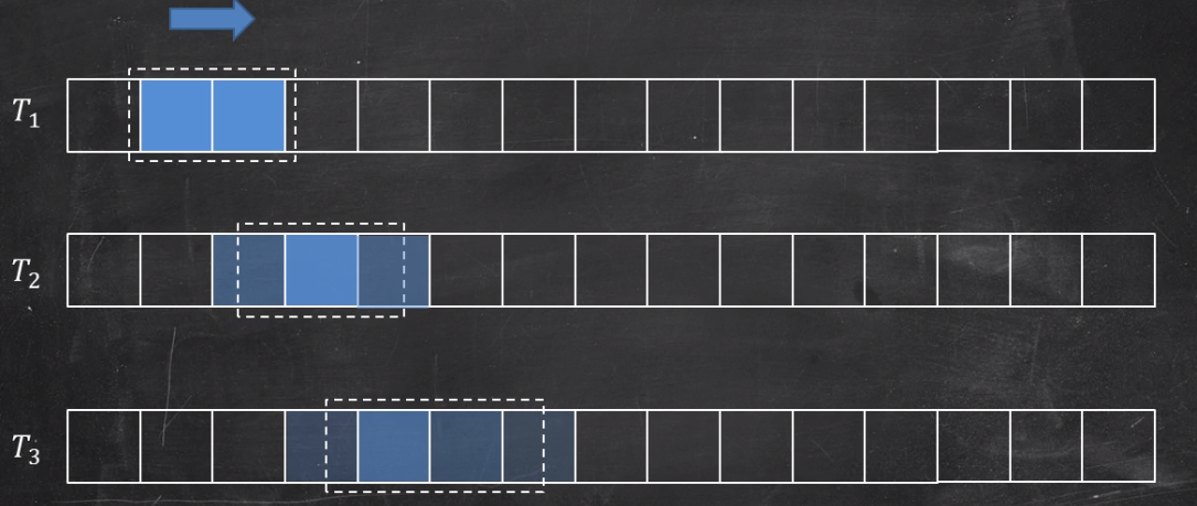
Mass conservation & Divergence
Mass conservation here means the amount of gas entering and leaving some arbitrary volume must be equal. It is the prerequisite if we want to use Navier–Stokes equations and Newton's second law to interpret the smoke movement.
In Houdini, the model of a single voxel is called MAC-Grid(Marker-and-Cell Method, developed by Francis H. Harlow, J. Eddie Welch in 1965). In the model, velocity plays a primary role in maintaining mass conservation. By default, the MAC-Grid samples scale field(such as density, temperature, pressure) in the center. However, for the velocity, each voxel samples its components from different three cell surface(see pictures below). 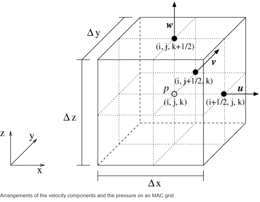
Picture from researchers Gate
At this point, velocity is used for defining the amount of matter entering and leaving the voxel. The velocity at the location where it was sampled defines how many matters enter the voxel; the velocity was sampled from where faces they leave defines how many matters leave the voxel. The difference between the input and output is called divergence. To maintaining mass conservation, we have to provide zero divergences for the whole simulation.

Fields and Euler viewpoints
After understanding all the aspects above, we can make some simple conclusions:
- The Basic unit in Fluid simulation is voxels
- Voxel Can contain some information to define how fluid moves
When we put all voxels together, the information from all voxels consists of a data flow, and we call it fields. Fields are the key that we use to control the entire movement of fluid in a specific space.
Depending on what kind of data we stored in voxels, fields have different types. In general, if we look at fields in data form, there are mainly two types of fields:
- scalar fields, which contains scalar data(such as density, temperature)
- vector fields, which contains vector data(such as velocity)
By combining all the fields, we can finally describe how fluid behaviors in our simulation.
The Movement
Now we have the container for store the data. The next question is, how can we utilize the data to approach a simulation?
The incompressible Navier Stokes equations
Navier-Stokes equation is an equation to tell us how the fluid moves, behaves, what is going on about the fluids. Everything that can change its shape to match the container can be described by using the Navier-Stokes equation.
There are two types of Navier Stokes equations. Houdini uses the incompressible Navier Stokes equations. Generally, the incompressible Navier Stokes equations have two parts:
In the equations:
- $\vec{u}$ means velocity (vector)
- $t$ means time
- $\rho$ means pressure
- $g$ means external force (uausally only gravity, so $g$ here.)
- $v$ means viscosity
The Mass conservation one tells the fact that the simulation in Houdini is under incompressibility condition, which is the zero divergences that we discussed before. In Houdini, the Gas Project Non Divergent node can be used to remove any divergent parts in fields.
The second one in which implying momentum conservation is a little bit more complicated, but generally, it is another form of Newton's second law. In this part, we can do a little modification on it.
As we know, acceleration is the time derivative of velocity. If we only leave the acceleration on the left of the equation and comparing to the equation we all familiar with, we could find something interesting:
From the picture above, it is easy to discover that the Momentum conservation part tells us fluid accelerates affected by forces and can be explained well by Newton's second law. Let's take a look at what is exactly on the right-hand side of the equation:

It actually can be divided into four parts:
- self-advection(velocity to velocity)
- viscosity(diffusion)
- external forces
- pressure
self-advection
As we mentioned, advection is the updating process of fields. Self-advection can be described as not only field drives the motion of the fluid, but also itself. For example, let say the velocity field causes the fluid moves, and as a result, the moving fluid will go back to update the velocity field too.
In Houdini, the Gas Advect mircoslover can be used for advecting fields based on an existing field. If we have some interaction between fields, The Gas Calculate node can be used to copy information from one field to another.
viscosity(diffusion)
The diffusion controls how velocity propagates from the source, and the viscosity is the key parameter to determine the propagation speed.
In Houdini, the Gas Diffuse node can be used for spread out the velocity field, and the Gas Viscosity node can be used for apply viscosity to the velocity field.
external forces
This part can be considered as a combination of all external forces, such as gravity. In Houdini, we can even put more force on it, like wind, drag. We can also add our custom fields to generate new force.
Pressure
the pressure is used for describing different pressure between high-pressure areas, and low-pressure areas generate a force to push the fluid move. The gradient of the pressure field represents the force. Of course, the force implies how fast the property changes in the field.
How Houdini Process it?
Since N-S equation hasn't been proved that it can't be solved(so far) analytically, Houdini used some numerical methods to approach the result. The method to solve the equation in Houdini is called splitting, that is, separate the equation in several portions, then solve each by using finite difference method. Generally, it has 3 steps:
- $ \frac{d\vec{u}}{dt} + \vec{u}\cdot\nabla{\vec{u}}=0$ this part is also called material derivative, it calculate how velocity changes due to the fluid motion.
- $ \frac{d\vec{u}}{dt} = g(f)$ this part calculates how velocity changes due to the external forces.
- $ \frac{d\vec{u}}{dt} + \frac{\nabla{\rho}}{\rho} = 0 \,\,\,\, \nabla{\vec{u}} =0$ this part provides the incompressiblilty condition to whole simulation.
Besides, we also need a place to store the simulation, and also a way to import our source. Thus, the whole process can be described as follows:

Pyro solver
The only difference between smoke solver and pyro solver is pyro solver has its composition model. It is easy to understand once we know how Houdini processes the fluid simulation.
Generally, the combustion model is a bunch of fields advects each other and manipulate the property inside the fields. You can see the general process as below:

Drawbacks of Pyro solver
The implementation of SideFX has some issues.
In some cases, you may find the smoke would rise in high velocities without high temperatures. For example, if you check the picture below, you may find the smoke in the middle keeps the velocity at a high level despite it already lost the temperature(the flame turned into the smoke already).
Another issue that can be also found is turbulence on the smokes. The turbulence just continues to break itself on the surface, that cause we have big mushroom effects on the fast-moving parts and make the smoke turbulence looks like it never coming from inside of the explosion. 
I didn't come up with any solution to the first issue by just tweaking the parameters on the pyro solver. For the second problem, it can be fixed by animating the turbulence. However, we can modify the fields to make the simulation more realistic.
Customize Pyro solver Based on smoke solver
In this customized, we are able to create everything for combustion based on the density field. The smoke solver will be used for the basic shape of the simulation, and the details will be added to the basic shape by creating and blending existing fields.
The basic idea is generating the density gradient field recursively, and blend it with current velocity field ever step. By doing this is we can obtain some benefits:
- We could get more details inside of the volume movement. The density gradient field indicates the movement direction, and it happens both inside and outside of the volume.
- By recursively computing the gradient field, we could get some fractal effects on volume, and that effect causes more details on volume without applying any turbulence.
- Because the movement is driven by density gradient, it is easy to know we will get low velocity when smoke is able to disappear(low-density cause low gradient), which is very natural.
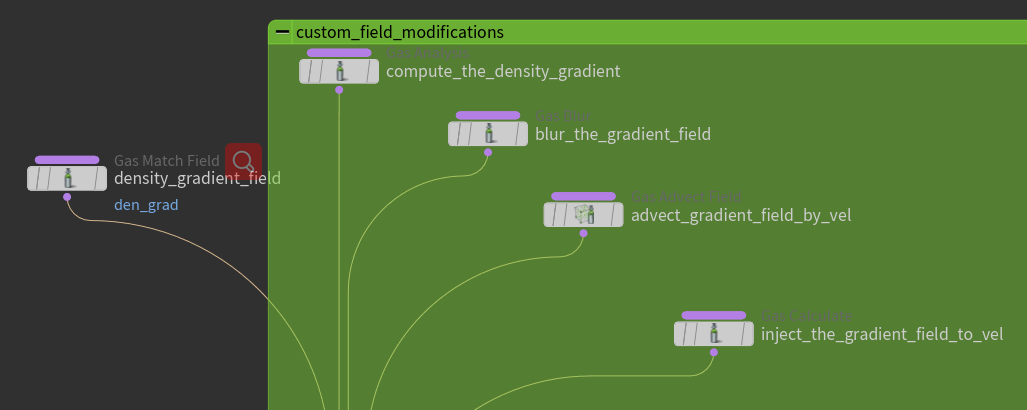
gerenal workflow for blending fields
It is worth to mention that the blending field operation can be implemented by using Gas Calculate node. Creating the rest of the steps is just as easy as we discussed before:
- creating a space for storing the fields
- modifying the fields in different ways(blur, Diffuse, Analysis...)
- Advect the target field by using the velocity field to make sure it has the correct behavior
- Blending the field with an existing field (Gas calculate can modify them both and do a specific calculation on two fields)
- keep zero divergence
- some cleaning work to save memory (Gas linear combination with zero coefficient)

Calculate the gradient of density
The first thing we need to build is a custom velocity fields. The new fields we will create is density gradient fields, and it will be blended with velocity fields finally.
Modify the gradient field
Adding the noise to the gradient field
Noise is one of the crucial methods that we can add details to the volume. In this case, the noise is applied to the gradient field directly by using the Gas Field Vop node. The node allows us to do some math computation inside the DOP like general VOP networks.
It is also good practice to normalize the field before adding any modification on it:
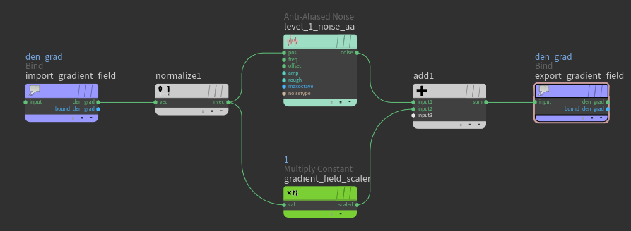
By adding the noise, every step the noise will apply to the updated gradient field and cause more random detail. To get more details, the updated gradient field is good to have portions above and below the edge of the field we got from the previous gradient field. At this point, Alligator Noise is a great choice.
Stacking the noise
For adding even more details, we can also stack multiple noises together as well. It is good to start with one noise to get a basic shape. Once we satisfy with it, we could add more noises to it to break the pattern into smaller pieces. Besides, we could also add the different offsets to each noise as well; it going to help random the details as well.
Separate density gradient field
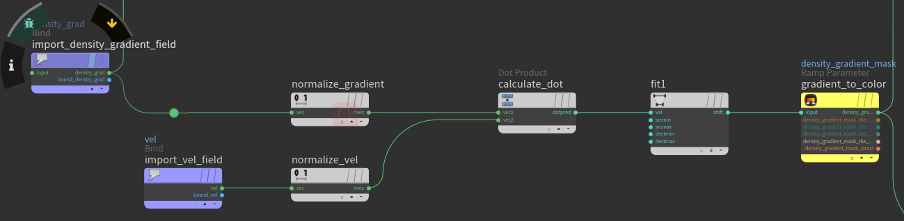
Sometimes it is good to have more control in different areas of fields. In this case, Adding different noise to the different density gradient field area would be a good idea. For example, when the source is staring to emmit, the speed and temperature are at a high level. A high-speed movement would cause less variation in the volume. Thus, it is necessary to isolate the fields based on velocity.
At this point, a dot-product can be utilized for the separation. The Gradient field of density implies both the direction and speed of the field. If we use it to make a dot-product with the current velocity field, the result could be between [-1,1]. The value which is less than zero will be in the opposite of the direction of the velocity and vis Versa.
This data can be used to isolate the gradient field. We can feed the data into a color ramp with two different colors(e.g., red and blue). Depends on the ramp, different colors can represent different areas through different color channels. Once the areas are accessible, those channels could be used as masks to the gradient field by multiplying themselves to the field.
On the other hand, it is also good to use the separated field to control the dissipation.
Curvature to Temperature
In this custom build, we are going to use the temperature field to represent the fire, and the temperature field comes from the curvature field of density.
The reason to use the curvature field to generate the temperature field is, it is easy to obtain the "cracks" between the large mushroom of volume. In real-world reference, the most high-temperature area comes from the "cracks":
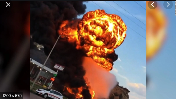
It is easy to isolate the cracks by calculating the curvature field. Those cracks have a higher value in the curvature field, thus we can pick them up by using the color ramp technique we discussed before. The selected curvature field is showing as the red area in the below picture, which is perfect for representing the temperature field: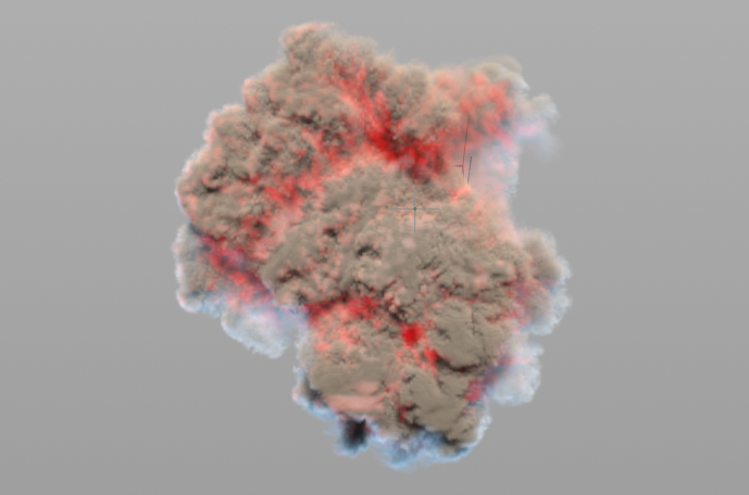
Adding blur on the curvature field would help make the cracks more visible. The Gas calculate node can be applied to turning the curvature into temperature.
Manipulating the temperature
So far we have injected the curvature back into the simulation as the temperature field. However, in the real world, temperature is related to velocity. Thus in our simulation, the data from the velocity field is the key to get the realistic movement of the flame, as it is going to be represented by the temperature field.
The basic idea is acquiring data from the velocity field as the temperature field first. Once temperature field moves, it is able to go back to cause the velocity field change as well. The loop will continue forever to drive the flame movement until it reaches a specific threshold, which can be defined by users.
It is also worthwhile to have three improvements for the loop:
- Using the fastest portion of the velocity field to create the temperature field, as the higher temperature causes faster movements.
- Adding the high-speed area to the existing velocity magnitude field(the result of the dot product between density gradient and velocity), so only the high-speed area is along with the density gradient will have a high temperature.
- Clamping the temperature to prevent it from exploding which is caused by extreme value.
